OK, you’ve just been assigned a new project. There’s a cell that’s in need of Monte Carlo variation analysis. You’re looking for 6σ accuracy – 1 failure in a billion. So you run the numbers, and you find that you’re going to need 5 billion separate simulations. Yes, that’s with a “B.” No, retreating to a less aggressive node won’t help; this number is independent of the number of varying parameters. Straight statistics. Yeah, this project is going to take… years.
So, of course, that’s not going to happen. What are your options instead? Well, one is simply to overdesign – make sure you’re so rock solid that you can sleep nights without all that simulation. Of course, this will likely use more area and power than is really necessary, but it lets you ship a product on time.
Another choice might be to make simplifying assumptions. Assume linearity. Assume Gaussian distributions. Assume the earth is a perfect sphere. (Or perfectly flat, if that’s your thing.) Without these assumptions, each simulation is independent of all the others. But by assuming, say, linearity, you have now related a set of simulation points. Two points define a line, and then you can inter- and extrapolate to get any other points along that line. You’ve now imposed some structure on your data set so that it’s more than just a random scattering of data points. And every point on that line is covered by the two simulations it took to define the line.
It’s like you’re creating a model for modeling – a kind of meta-model. You’re doing what we in the semiconductor world do so well: abstracting. Imagine if we had to model all our circuits at the SPICE or <gasp> ab initio level. Not tractable. So we abstract at each layer. Instead of simulating all points, we can simulate some and then calculate the rest based on the assumptions – that is, the model – that we impose on the data.
Which is great, in concept. But here’s a question: how do you know that the assumptions you’ve made are correct? If you’re the first guy to do this, you really don’t know. You have to try it out and see if it works. Once certain assumptions establish a track record, then you assume that your assumptions are correct, largely because similar assumptions have worked in the past.
But what if you’re wrong? Or what if the analysis you’re doing depends on explicit process-related inputs and the latest process node has raised 2nd– and 3rd-order effects that didn’t matter before? You can’t explore that by imposing a model that assumes that they still won’t matter.
Here’s the problem: creating a model at this level, as opposed to a collection of unrelated simulation results, can be really helpful. But we, as humans, have a limited set of constructs to use in this model. Specific behaviors like linearity; distributions that fit nice, well-behaved equations. That’s pretty much it. And there’s nothing that says that nature has to follow that limited set of choices.
But help is on the way. While humans will have a hard time doing a nuanced meta-model, there’s a new contributor to the solution that can do a better job than we can: the Machine. And here’s the key: the machine doesn’t start by imposing assumptions; it lets the data itself establish the assumptions that naturally reveal themselves, even if we would have no way of articulating the assumptions in words or in a convenient symbolic equation. And, really, if the assumptions arise from the data, then they’re not assumptions. They’re observed patterns.
Put the Machine in Charge
We hear about machine learning all the time, but usually in the context of AI and the Internet of Things and Big Data in the Cloud. We in EDA haven’t had to deal with it so much. So, as a quick refresher for anyone new to this, there are a couple of ways to do machine learning: supervised and unsupervised. Supervised means you have a starting data set that’s used for training. Unsupervised means the machine learns on-the-job – which means it needs some way to know whether or not it’s making a mistake so that it can feed that result back and improve its model.
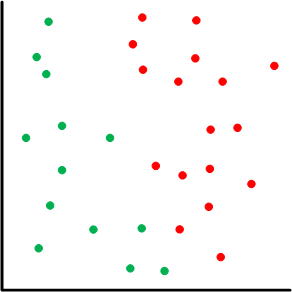
Let’s break this all down a bit, looking at the notion of the “model” first. A graph like what follows is often used to illustrate these principles. You’ve got a bunch of data points, and, in a simple pass/fail scenario (like a shmoo plot), some (green) are pass and some (red) are fail. The challenge is to come up with a model that lets us establish whether some new data point – one that’s not in the original set – is a pass or fail.

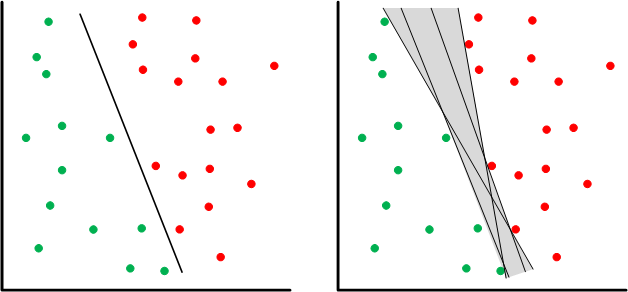
We’re more or less looking for some way of separating the passes from the fails. This is a point in the game where we may still impose some structure. We could, for example, go for a linear “separator” like what follows. On the left we see a line that more or less splits the difference between the two groups of points. That could be our model. But there’s nothing pinning that specific line down; it’s an artifact of the machine-learning algorithm. There’s a range of lines (shown on the right) that would be equally valid for this data set.

If you’re training with a fixed data set, then you end up living with this ambiguity – or you get more data to help narrow down the range of options. But with an on-the-go learning mechanism, the machine can make predictions and then test them – creating new data points to fill in voids.
From a simulation standpoint, you can start with a depopulated graph and run a simulation. Let’s do two points, since then you have two things to separate. The machine’s algorithm can come up with some separating line based on its algorithms, but that line will probably be wrong. So the machine picks a new point and, based on that line, predicts the result – which will also likely be wrong since the model is so unrefined. It finds that out by simulating that point to get the real answer. Seeing that it’s wrong, it adjusts the line so that it works with the new data point. And then it repeats this predict/test/correct cycle until predictions and actual results start to align within a certain margin.
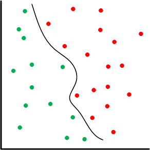
There are lots of knobs that we can dial up to make this more or less efficient or accurate. For example, it’s entirely likely that a line may not work as a separator; perhaps something more polynomial in nature – or whatever. Yes, we’re imposing structure again, but it allows for the machine to come up with a much better fit than we could do manually.

You can also well imagine that you could pick new points completely at random, but then you might spend a lot of time simulating points that aren’t in question. If you’re zeroing in on the curve above as a separator, then simulating new points way out to the right probably wouldn’t be useful. Picking new points near the separator, on the other hand, is helpful for tuning the model until predictions are all accurate within the margin you’ve selected.
Solido’s Machine Learning
Solido has announced a machine-learning initiative – a mixture of new products and internal capabilities – and, depending on the application, the drawings above are a fair, if over-simplistic, representation of what’s going on.
Let’s take that 5-billion-simulation problem. Conceptually, you simulate various data points, and, at the point where you can make predictions, you keep generating new data points and adjusting the model until your predictions zero in. If you pick your new data points judiciously, then you concentrate on the simulations that matter. Once your predictions work, you now have a model to use for new points rather than having to simulate the new points. And, according to Solido, the 5-billion-sim problem can be solved with around 3000 simulations instead.
To be clear, you still need the 5 billion points to establish 6σ. It’s just that you don’t have to simulate all those points. You simulate a small subset, letting the machine detect the pattern, and then you can calculate the rest of the points – much faster than simulating them.
This is one example of the output of what Solido is calling ML Labs. They’ve built up a general machine-learning capability that they can use to develop new tools. The Monte Carlo scenario we’ve been discussing is handled by their Variation Designer tool.
They’ve also announced their ML Characterization Suite, consisting of a Predictor that generates models at new corners from an existing set of corners and a Statistical Characterizer for statistical timing models achieved with a minimal set of simulations.
But the thing with ML Labs is that Solido gets contacted by customers who have a problem to solve. Those customers may also have lots of data – but no good way to analyze it or present it. So they ship it to Solido, who use their own internal machine-learning tools to develop the desired tool – which can then be sold to the general public. I was a bit surprised that semi folks would be willing to share proprietary data that would result in a tool that could help their competitors, but apparently their needs are urgent enough to where they’re ok with that.
I also asked why they didn’t simply make the machine-learning tools available as a product so that customers could develop their own proprietary tools. They responded that there hasn’t been demand for this; folks are happy to have Solido do the work and turn around a new tool.
So that’s how machine learning is impacting the EDA world. Something tells me we’ll be seeing more of this wherever large data sets are found.
More info:


What do you think of Solido’s machine-learning approach to developing new tools?