We hear a lot about artificial intelligence (AI) these days. The mentions are typically delivered in acronym salads that include machine learning (ML), deep neural nets (DNNs) and the other various NNs (convolutional – CNNs, recurrent – RNNs, etc.), and a pile of other technologies. Many of these are accessible only to specialists; the rest of us nod our heads sagely, pretending to understand, hoping no one calls us out.

But at this year’s Linley Spring Processor Conference, Linley Gwennap did a keynote that looked at many of the technological vectors that are being traversed and what’s pushing them in that direction. The presentation took a step back and focused on some high-level concepts underpinning what makes AI work.

While his focus was on how the technology was evolving, I was also intrigued by the collocation of so many fundamental concepts – some going by names we non-specialists don’t necessarily use on a daily basis. So, while I’m not going to parrot the specific points made in the presentation (you’ll have to get the proceedings for that), I thought it useful to walk through the basic notions, in the hope that any new nuggets you find for yourself will be helpful.

The order in which I’m going to present these in has nothing to do with anything other than the rough order of their appearance in the presentation. So, with that, let’s take a look.

Perceptron

This term actually wasn’t a part of the presentation itself. But it’s such a fundamental concept that it’s worth starting here. It’s a word that doesn’t show up often outside specialist circles (at least as far as I’ve seen). As a result, when you do run across it, it can throw you – or send you running to the web — which is where I went when I first encountered it.

The perceptron came about as an alternative to the neural-net model that more closely resembles what happens in our brains: the spiking neural net, or SNN. In SNNs, data is encoded using spikes. Either the frequency or timing between spikes is used for that encoding. The math used for inference processing is simple, but this is hard to manage for standard supervised learning. There’s no easy way to take derivatives or do back-propagation, for example. And, so far, they don’t scale well.

So the perceptron, while less brain-mimetic, makes it easier to accomplish practical ML. The idea is that, if a function crosses a threshold, it gets classified within some category; otherwise it doesn’t. The result is binary that way.

Mathematically, it looks like this:

Here w and x are vectors, with w representing weights and x representing the inputs (or activation*). The b is a “bias” or threshold. The operator you see there is the dot product (which is ancient history for me), meaning that it’s the scalar result of the following function for vectors of length n:

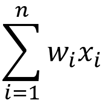
Yeah, basic review, but one thing becomes screamingly clear from this: you multiply a bunch of vector entries and add them all together. In other words, this is where the popularity of the multiply-accumulate (MAC) function comes from. Of course, you hear a lot about matrices rather than vectors, but matrix multiplication merely builds on this, with columns and rows acting as the vectors.

Systolic Arrays

This is a mysterious-sounding notion that, for me, invokes arcane math and science that hasn’t made it to the mainstream enough for this to be a common term. Maybe that’s just me, but it turns out that, at least conceptually, this is a natural notion for neural nets – and matrix multiplication in particular.

We talked about a vector dot product, but, in reality, we’re not talking about vectors, which are one-dimensional arrays. We’re not really even talking about matrices, which are two-dimensional arrays. We’re talking about multi-dimensional arrays, aka tensors. Whence the framework name TensorFlow.

In reality, tensors get broken up into multiple matrices for calculation (in the way that matrices get broken up into rows and columns), so the problem degenerates to matrix multiplication. Using a basic CPU for that is pretty cumbersome, since you re-use the computing engine over and over for each of the n x m MAC calculations. That’s why GPUs or DSPs with high parallelism do better.

Even so, with parallelism that’s less than the sizes of the matrices, you end up bringing in inputs and weights for the parts you’re going to work on; they come from memory. Your partial results then have to go back into memory, where they’ll be recalled later when the processor gets to a future part that needs those results. That memory movement is a huge time and power waster.

Systolic arrays are one approach to making the math more efficient. You can think of generic systolic arrays as matrices of functions, or rather of a single function, since they’re typically monolithic in that way. How the “entries” in the matrix are interconnected can vary, but, for our purposes, a typical connection scheme is shown below.

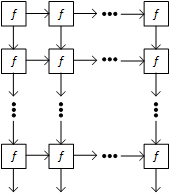
The tendency of data or cumulative operations to flow through the array gives rise to the name systolic. It’s by analogy to the pulses of blood that course through our arteries. You may be familiar with it as the first number in your blood pressure reading.

For our application, the function f in the figure above would typically be a MAC function. One way to accomplish this is to store the weights in their respective cells in the array. Such a processing element would look like the following figure (where PSoP stands for partial sum of products from the cells above).

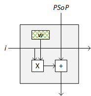
In this case, all the weights are preloaded, and each input column from the left can be available simultaneously to each array column. You then cycle through the input columns. You could operate this such that the sums happen combinatorially, and, given time for the sums to propagate down, you’d end up with complete sums of products at the bottom of each array column.

Rather than preloading weights, you could stream weights in from the top and inputs from the left. Propagation right and down would happen with each clock cycle. Both input and weight matrices would be fed, with suitable clock-cycle delays, into the left (for inputs) and the top (for weights) (although, mathematically, you could exchange the weights and inputs in this view). The element here could look more like this:

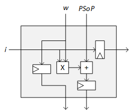
The end result would be that each array cell would contain the entry for the product array.

Google is said to have put together the first serious use of a systolic array in their tensor processing unit, or TPU.

In-Memory Computing

Given that data movement is such a problem during inference, yet another approach has been proposed: using memory itself for computing. This, of course, assumes an array of memory cells for computation. There are a couple of approaches to this, the most direct being an analog one.

You may recall our discussion on RRAMs (or ReRAMs) a long time ago. The memory works by forming filaments between two electrodes. Thinking in a binary way, the presence of a filament is one state; the absence is the other state.

But here’s the thing: you can have partial filaments. The conduction will be proportional to the “amount” of filament in place. So you can use this as an analog memory. If you store the weights as the memory and then apply the inputs to the memory as an address, you’ll get current through each cell inversely proportional to the resistance in the cell – or proportional to the conductance.

So you store the weight as a conductance, not a resistance. If you then sum all of the currents in a column, you’ve got a sum of products.

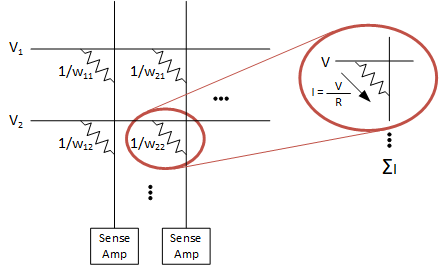
We discussed in-memory computing in much more detail in a piece from earlier this year, including the fact that, if you binarize the numbers, you can potentially save lots of power and area. Yeah, I know, we go from binary to analog back to binary. But the thing is that the first “binary” is used to store a fixed-point number; moving to analog effectively stores a real number; and the last “binary” stores a binary number. So it’s not like we’re going backwards.

Suppressing Zeroes

These matrices can be pretty sparse. In fact, one optimizing technique is specifically to keep the matrices sparse. That means that there are lots of zero entries (or near-zero entries). These don’t contribute at all (or, if near-zero, appreciably) to the sum of products. So why calculate them? Exactly! Don’t calculate them; suppress them. We saw an example of this earlier in coverage of Cadence’s neural-net accelerator.

Bfloat Numbers

Next we look at a new real-number format largely being used by Intel and Google. It cuts the length of a 32-bit floating-point value in half. Yeah, there’s a standard 16-bit floating-point number already, but it can’t express the same range of values that a 32-bit floating-point number can.

32-bit numbers use an 8-bit exponent and a 24-bit mantissa (or 23 bits plus one sign bit). The exponent gives you the approximate range of numbers you can express (±28), while the mantissa gives you the precision available within that range.

If you want a standard 16-bit value, the standard format has 5 exponent bits and 11 (or 10 + sign) mantissa bits. The problem here is that you can no longer express numbers in the 28 range; you get only ±25 – literally off by three orders of magnitude.

The bfloat format is also 16 bits, but it keeps the 8-bit exponent used in the 32-bit version and simply shortens the mantissa to 7 bits. That means you can still express (roughly) the same range; you just do so with less precision. Obviously, this format doesn’t comport with standard math libraries, so converting to and from integer values has to be handled on a custom basis. But it provides for faster computation and less memory use.

Activation Functions

Finally, our formula above defining a perceptron takes the dot product and then decides, based on a desired threshold, whether the result is 1 or 0. In fact, the bias b in the perceptron equation reflects a non-zero threshold. But how do we take this sum of products and decide whether or not it meets the threshold?

An obvious way to do it would be to apply a step function to the result, with the step occurring at the threshold value. But, for training purposes, you need the ability to take a derivative and to back-propagate (just as we saw when using a perceptron instead of an SNN).

If you look at the Wikipedia page on activation functions, it lists a huge number of possible candidates. More common are sigmoid functions (so-called because of their s-like shape – although, to be fair, it’s not a sigma-like shape…), and, for that differentiability thing, the hyperbolic tangent is a popular sigmoid.

The important thing about these functions is that they’re good candidates for acceleration, since whichever function is chosen will be used a lot.

And that will wrap up this survey of neural-net notions, at least as I understand them. As neural nets complete their exploratory life and enter into a standardized life (if that ever happens), much of this may be abstracted away. For now, these are useful notions for anyone trying to dip their toes into practical implementations of AI.

*You’ll sometimes read that the output is an activation. That’s because the output of one layer is the input to the next layer.

More info:

2019 Linley Spring Processor Conference proceedings (requires submittal of a form)

Video of Linley Gwennap’s presentation (no registration required; in four parts)

Sourcing credit:

Linley Gwennap, President, The Linley Group