A few weeks back, we tackled the concept of a single-electron transistor (SET). And we saw how they could be arranged in a hexagonal form for use as a non-volatile programmable fabric. The whole topic originated for me in an ICCAD paper that discussed EDA algorithms for implementing logic in such a device. Well, before discussing that, we needed to introduce SETs. So, having done that, we now return to the originating topic: how do you take random logic and implement it in a SET fabric?
This could descend into the realm of intricate minutiae (details make the difference between algorithms that work and ones that almost work); I’m going to delve in only so far for flavor. I’ll refer you to the original paper (link at end) for the remaining bits. But… yeah, it’s gonna get moderately wonky.
It’s also important to keep in mind that what we will discuss is only combinatorial logic. It’s early days for SETs – they’re far from commercialization, so full system implementation is a ways away yet. I checked in with all of the major EDA guys – no one is working on this in any serious way. It’s still considered to be too researchy.
So why even put time into it now on these pages? I guess because it fired my imagination; it seemed different enough from what we’re used to that it was nice to spin up a whole new section of my brain to think about this. Hopefully it does for you too.
SET review
So… as a quick review, let’s reprise a couple of quick relevant notes; I’ll refer you to the prior article for a better understanding of the underlying whys and wherefores.
- A SET allows one electron to pass from source to drain if the gate so directs.
- SETs can be arranged into a hexagonal fabric such that a single electron can be routed from one end of the fabric all the way through to the other end.
- Each horizontal row along the “angled” hexagon facets corresponds to a single variable. The SET on one branch reflects the “true” value test; the SET on the other branch reflects the “false” test. Vertical lines are shorts.
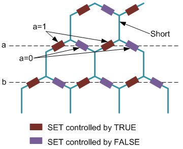
- A function qualifies as “true” (assuming active-high logic) if an electron can find a path through the fabric.
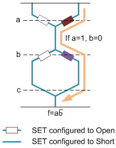
- A simplified graphic notation is used (which we will simplify yet further for algorithmic purposes). It’s slightly more efficient than the figures above. The following figure is equivalent to the prior one. The numbers on the variables (a1, a2, etc.) serve only to identify specific nodes in the fabric; they’re not different variables.
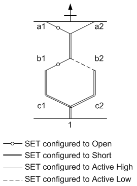
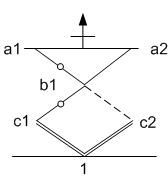
The graphic simplification we will make gets rid of the shorts that are always shorts: the vertical lines. The resulting diagram looks like diamonds more than hexagons and is therefore less reflective of the physical arrangement, but the abstraction allows more focus on what matters. Here again, the following figure is equivalent to the prior one.
Finally, we talked about a couple of constraints (granularity and fabric) last time; we’ll return to those, but there’s one even more fundamental constraint that we didn’t discuss: when the fabric configuration is complete, it’s important that one, and only one, path through the fabric be activated at any given time.
That’s because we’re talking about incredibly small currents that need to be detected – the smallest current possible, to be specific: a single electron. Having multiple paths active will completely muddy that measurement up, so it’s not allowed.
First constraints: one true path and planar
Ok, with those preliminaries out of the way, let’s look at how you implement logic on one of these puppies. As noted, this arrangement looks suspiciously like a binary decision diagram (BDD). At each level, we’re making a true/false decision and moving either to the left or to the right. BDDs will be pretty familiar to EDA types; they’re less so for the rest of us (hence the basics here).
BDDs tend to get simplified to “reduced order” BDDs (ROBDDs). This process, to me, is akin to going from a canonical sum-of-products (SoP) Boolean form to a minimized Boolean form. They’re equivalent, but one is more efficient – if more ad hoc in form.
So, for example, the following BDD can be simplified to the equivalent ROBDD by dropping variable nodes that don’t actually do anything (like b2 and c2) and merging nodes where possible (d1 and d2).
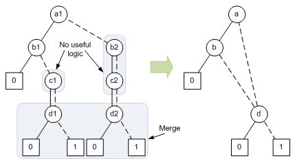
The original BDD looks a lot like the SET fabric situation, but there’s a critical difference: a BDD doesn’t have to be planar. In other words, it can have lines that cross each other – something that’s not possible in a SET fabric. An example of part of a non-planar BDD, shown in the paper, looks as follows:

Because a BDD (or ROBDD) has this fundamental difference from SET fabrics, early algorithms transformed the BDD into sums of products and then worked from the textual product terms to find a mapping on the SET fabric.
But the Michigan/Shanghai Jiao Tong/Tsing Hua team noted that, by moving from the graphic BDD to the SoP form, you sacrifice useful structural information inherent in the BDD. So their approach is to transform the ROBDD into a planar BDD that can be directly mapped onto the fabric. They abandon the transformation to SoP form entirely. This has resulted in some more efficient implementations.
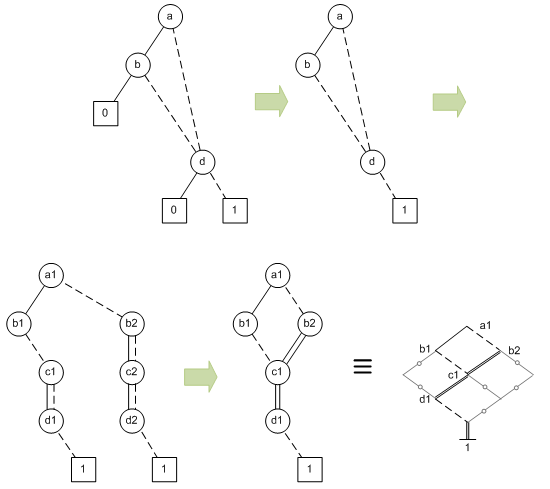
Ironically, the first steps they have to take on the ROBDD serve to reverse some of the steps that turned the BDD into an ROBDD. Those include:
- Pruning 0 nodes and associated edges, focusing only on true- or 1-oriented logic (the rest remaining implicit).
- Repopulating all variables; where true and false decisions have the same destination, turn that into a short.
- Merging identical nodes (they have to be identical for all logic below).
These steps are reflected in the next figure.
But what about non-planar BDDs? This results in some logic replication. So, taking the non-planar example from further up, you have to duplicate the destination node that causes the crossing. That means duplicating any downstream logic too.
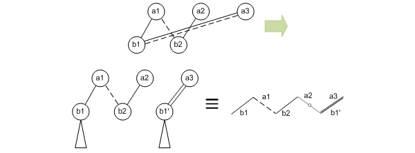
If you can place identical nodes next to each other, then they can be merged. It would be really nice if we could swap a2 and a3 up there so the b1 and b1’ nodes would be next to each other and then could be merged. But that would screw up the a1-b2 line, making it necessary to do different reduplication. So it doesn’t really help here; it can in other cases.
Next comes a step where conflicts are resolved. Mapping may try to place two nodes in the same place. These conflicts are an artifact of the detailed mapping process. If we look at it as humans, we might simply say, “Duh, don’t do that.” Computers have fewer such insights. (Some future work might create a conflict-free mapping that makes this step unnecessary.)
So the following example, from the paper, shows that two logical nodes, c2 and c3, might end up being mapped to the same place. Now… if those nodes were identical – including all downstream logic, this might be efficient. But if not, then this is a no-go. So you have to spread things out to make room so that c2 and c3 can each have their own nodes.
There are a couple of ways of doing this; one involves adding an entire row; the extra row doesn’t do anything except let the conflicting nodes separate. There’s another way to do it if the conflicts happen to occur at the edges of a row; that’s a special case that doesn’t require a new row insertion (I haven’t illustrated this one).

Remaining constraints: fabric and granularity
So at this point, we’ve transformed the ROBDD into a planar BDD, and we’ve met the two most important constraints: one true path and planar. Now we need to address the two remaining constraints: fabric and granularity. Frankly, these get more intricate than I really want to tackle here, but let’s review why these are necessary and then abstract how it’s solved.
In this piece, we haven’t been paying attention to whether “true” branches come out to the left or right. Mostly we’ve had true out to the left and false out to the right, but that’s probably biased by BDD convention. In reality, up to this point, there’s nothing to stop us putting any branch in any direction. That’s particularly useful if two nodes – one the outcome of a true test, the other of a false test – share the same resulting node.
But the underlying SET fabric places limitations on this. It’s a specific result of fabric design decisions as to which lines to connect to the true version of a variable and which to the false version. As we saw last time, there’s the standard “symmetric” version, with all nodes the same; there’s the “mirror” version, where the arrangement reverses in between; and there’s any other combination you want. The algorithm in this paper assumes that each row is consistent throughout, but that different rows can have different arrangements.
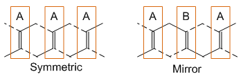
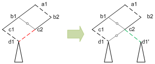
So, if we have a symmetric fabric, then the convenient arrangement on the left below will not work. It’s nice because the node d1 can be shared, but in order for that to happen, the branch from c2, which is a false test, has to go to the left – a no-no with a symmetric fabric. Instead, node d1 (and its follow-on logic cone) must be replicated. This consideration works itself into the mapping algorithm.
Finally, there’s the granularity constraint. You may recall that this originates in an attempt to save metal lines. For highest granularity, each decision point – which is to say, each SET – can be programmed to be active or open or short. But that results in a lot of metal lines for programming access, so architects consider sharing nodes – doubling or even quadrupling up. This means that shared nodes have to be programmed alike, which makes some combinations impossible.
So, for example, programming two SETs identically with one line means that the SETs must either both be active (whether true/false or false/true is determined by the fabric), both short, or both open. We can’t have an active-high line coming out the left and an open coming out the right, for example.
While the fabric constraint becomes part of the mapping algorithm, the granularity constraint is handled as a modification after the initial mapping to expand or fluff out the network, allowing only legal combinations. From the example below, given by the authors, this seems to chew up quite a bit more fabric than would be necessary without the constraint; that’s the price paid for the more efficient programming infrastructure.
In this example, you can see the illegal combination (red on the left); in the expanded network, the original logic lines are shown in green. All other lines are there simply because they have to be, due to the constraint (as indicated by the maroon markings).
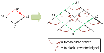
For instance, in the node between a1 and b1, there’s a false branch that then goes to a node with two opens. In other words, it does nothing. But because the left branch is active, the right branch has to be as well – and so the following open branches ensure that the unneeded false signal goes nowhere.
OK, that’s it, I promise. Wait, where did everyone go? Come on… this isn’t that dull, is it? I guess for me, this makes up for all the times I saw crazy-assed quantum math and freaked out. This is my kind of math.
So let’s pull ourselves up out of the muck and take stock. The intent here is to give a flavor of what EDA tools will be required to do if or when SETs ever become a thing. Specifically, if they become a thing in programmable fabrics like this. (Who knows, they might become manifest in a completely different arrangement.)
And… this is likely to be the last you see of SETs for a long time. Yeah, maybe not something you’ll be using next week, but consider this a flight of fancy into what logic might someday look like.
We now return you to stuff that matters next week.
More info:
BDD-Based Synthesis of Reconfigurable Single-Electron Transistor Arrays (behind a paywall)




What do you think of this algorithmic approach to fitting logic into single-electron transistor fabrics?