It’s been introduced as nothing less than a new way of computing certain kinds of problems. It’s another approach to computing more the way the brain does it than the way Mr. Von Neumann does it. Which is to say, using orders of magnitude less power than Mr. Von Neumann would consume. (Yes, given a chicken in every pot and a nuclear reactor in every backyard, Mr. Von Neumann can do most anything…)
A recent announcement by Knowm (pronounced like “gnome”) brought some renewed attention to their AHaH Computing paradigm. Before addressing what that means, just a heads-up that this is not obvious stuff; if this is going to become the new normal for certain types of computing, then it’s going to have to either get easier to understand or be completely abstracted away. We’ll come back to the specific announcement, but in order to provide the context, let’s first attempt an extremely cursory review of just what the heck they’re talking about, to the extent that I can decode it.
There’s a very thorough paper that lays out the whole concept, although it may be better suited to those already involved in this stuff. If you, like me, arrived at the party long after the cake had been cut, then it’s much harder to understand. There are lots of references to other natural phenomena, like the branching of rivers and a proposed 4th thermodynamic law, but they initially seem like analogies more than actual proofs. Unless, of course, you’re already steeped in this stuff. Or maybe it’s just me…
To be clear, lest I sound like I’m casting stones here, Knowm has produced an unusual number of documents and videos to help educate folks, so they’ve put in a lot of effort. But it’s a serious time commitment to absorb it all. And, while it may be sufficient for their audience, it’s still possible for the rest of us to go through it all and still have some holes in our understanding.
First, let’s tackle “AHaH”: it stands for “anti-Hebbian and Hebbian.” (And yes, they pronounce it like, “Ahah!”) I know, that might not have helped a lot. It’s all about how you implement learning. Hebbian learning tends to reinforce the current state at the next read (stabilizing); anti-Hebbian tends to mean that the state is likely to change on the next read (dissipative). We’ll come back to specifics on this in a bit; I just didn’t want you wondering throughout this article what it stood for the way I wondered during my research.
The broad idea is that any branching phenomenon – veins in a plant, rivers emptying into a delta, etc. – acts in a manner similar to an AHaH node. Let’s say something branches into two: those two branches compete for whatever is flowing (water, nutrients, etc.). And through this competition, the systems adapt in a way that maximizes energy dissipation: this is the proposed 4th thermo law.
For computing, they implement this notion not by harnessing rivers, but by using a configuration of memristors. We discussed memristors some time back; they’re considered (not without controversy) the fourth element to complete the set of fundamental passive components (resistor, capacitor, and inductor being the other three). The interesting thing about them is that they relate the time integral of current (which is charge) to the time integral of voltage (which is called flux, by analogy to magnetic flux, but involves no actual magnets).
d? = Mdq
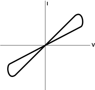
In other words, the device remembers (“remembering” being a loose rendition of “takes the time integral of”) the history of current flow. The IV curve takes on a “pinched hysteresis” look as shown below. You’ll see that, depending on where you are on the curve, you may have one slope or another. Or, critically, at the ends, you may be somewhere in between. The slope is the resistance, and so this device can attain one of two static resistance values, and this becomes the state and the mechanism for memory.

(Yes, I know… at the edges as you round the corners you’ve got negative resistance. This is abstracted; the IV curves for measured devices aren’t quite so pretty, although snapback phenomena do usually involve narrow negative-resistance regimes.)
The “official” symbols for a memristor are the first two shown below; the bar on the second one indicates polarity. Knowm actually prefers a different symbol, which they say is easier to draw and is reminiscent of the pinched hysteresis look. I can see that this is easier to draw by hand on a whiteboard, but it’s dramatically harder to draw properly on a computer, so I’ll stick to the other. I’ve approximated it below because I don’t have the right drawing tools (or the time with less professional tools) to truly do it justice (it should look like an infinity sign, not two abutted ovals).

There are a number of different ways to hook these things together to create AHaH nodes, and the paper makes reference to variants using an opaque system of numbers. The simple example we’re going to look at is what they refer to as a “2-1” two-phase circuit.
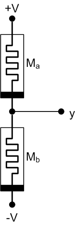
The basic node involved in this circuit is the voltage-divider-looking thing below. The competition comes from the evolution of the resistances – or, flipping it to the way Knowm looks at it, the conductances – of the two memristors. The total resistance across the two remains constant; the battle is between which node gets to conduct more current. If left running, it will evolve to a steady state with both conductances the same and the voltage at y equaling 0 V (since they both conduct the same current and, over time, attain the same history). But that’s not how we use it.

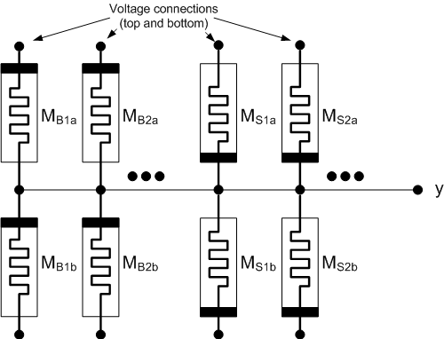
These nodes can be combined into a synapse as illustrated below. There will be, in general, two categories of node. You have bias pairs (labeled “B”) and input pairs (labeled “S” – probably for “spike”). The bias pairs set the basic voltage at any given time; the inputs are where encoded “spikes” are presented for learning. Note that the bias pairs are inverted from the input pairs. Upper memristors are labeled “a”; lower ones “b”.
The input pairs may be active or inactive. If inactive, then the top and bottom connections float. If active, then they’re connected to the voltage sources. This sets us up for the two possible operations: reading and writing. Reading measures where the node is at the moment – with a catch. Writing implements a… oh, let’s call it a teachable moment.

When nothing is happening, the voltage connections are disconnected and there is no current. Good for low power, and, because the memristors are non-volatile, the system state is preserved. The catch when reading is that you run current, and running current means that the memristors’ history evolves, potentially changing the conductance values. In other words, reading is slightly destructive (much less so than with a DRAM cell – if “perturbative” were a word, it might be more appropriate). So steps must be taken to “repair” this read damage.
There’s another catch in the whole thing: if you keep using the circuit in this configuration, everything moves in one direction, and, eventually, the memristors “saturate” at their maximum (or minimum) conductance. So steps must be taken to avoid this.
The basic read operation applies any spikes by placing voltages +V and –V on all bias and active input pairs and then measuring the value at node y. If you follow this by another read, you do the same thing – except that you invert the voltages. Meaning that the controller/driver must be aware of how the prior read was done to make the next read happen correctly. By flip-flopping successive reads, you both repair read-induced “damage” and avoid saturation. (The saturation solution is, to me, reminiscent of the disparity concept in 8B/10B encoding.)
Writing is similar, except that the y output now becomes an input. How this is done depends on whether the learning is supervised or unsupervised. Supervised learning means that the system is trained with specific patterns; unsupervised means that the system evolves on its own. If supervised, then node y is forced by an outside source to some value consistent with the training pattern.
If unsupervised, then node y is used as feedback by way of a digitizing function. If y is above zero, then you apply –V; if below zero, you apply +V; and, if zero, you apply zero. Note the tendency to work counter to the present state – again, keeping the memristors out of saturation. This digitizing also provides node y with a double function: the digitized version gives a “yes/no” answer, while the analog value gives a confidence level.
Again, flip-flopping successive writes is the order of the day. There are a variety of “instructions” used to manipulate this circuit (both flipped and flopped versions), but, given that it’s going to take me more hours to think this through in detail for a thorough understanding, I’m not going to pretend that I understand it any better than I do. I’ve read and reread this stuff in search of the elusive “ahah” moment; it eludes me still, although I’ve felt it brush by me on a couple of occasions.
You can probably see where my early comment about making this stuff more understandable (or entirely opaque) comes from. I can’t imagine training the bulk of the world’s software engineers to think in these terms unless we raise a whole generation of new coders and give them memristors to play with as infants so that this stuff is natural to them. (“Daddy, read me again that story about the little memristor that saturated and made the nuclear power plant explode!”)
The intent here was to give a flavor of this whole scheme. There’s lots more to dig into with respect to figuring out which of their instructions implement Hebbian and anti-Hebbian learning, scary-sounding concepts like state attractors (keep your kids away!), and other mind-bending notions. Having grazed the surface (to better or worse effect), we return to the announcement.
The release contained two elements. One announced the availability of new memristors. Memristors are made with a variety of metals, and, having started with tungsten, they announced tin and chromium as well.
But Knowm is also well aware that tools and models are needed for further work, and the folks designing such things need data. So Knowm has released a raft of data from their work so that others can use that in their own development work.
Such tools and models will ultimately be necessary to make this stuff accessible to your average Joe and Jane who just want to write their dang program.
More info:


We only scratched the surface here, but do you see promise in Knowm’s neuromorphic machine learning approach?